Applying sequence stratigraphy in petroleum geology: from systems tracts to sweet spots

A well log tells you what happened at one point. A sequence framework tells you what to expect between and beyond the wells, because it ties every package to a stage of the base-level cycle and therefore to a depositional environment with known grain size, sorting and geometry. That is the only defensible basis for extrapolating reservoir quality into undrilled acreage.

• Reservoir — regressive tracts (FSST, LST, upper HST) concentrate coarse, well-sorted, shoreline-attached sand bodies and turbidite lobes.
• Seal — transgressive and condensed intervals (TST, around the MFS) supply laterally continuous shales.
• Source — the same condensed sections carry the highest organic content and the strongest gamma-ray response.
• Trap geometry — sequence boundaries and their incised valleys create stratigraphic traps independent of structure.

Because reservoir, seal and source all follow from the same cycle, a correct tract subdivision immediately ranks intervals by prospectivity — before any petrophysics is done.

The first hard test of an interpretation is core. Every plug carries a depth, so it inherits the tract assigned to that depth by the log interpretation (or, at the well location, by a seismic zone). Colouring a porosity–permeability crossplot by tract turns a generic cloud into separate populations, and reservoir cutoffs turn those populations into net-reservoir shares.

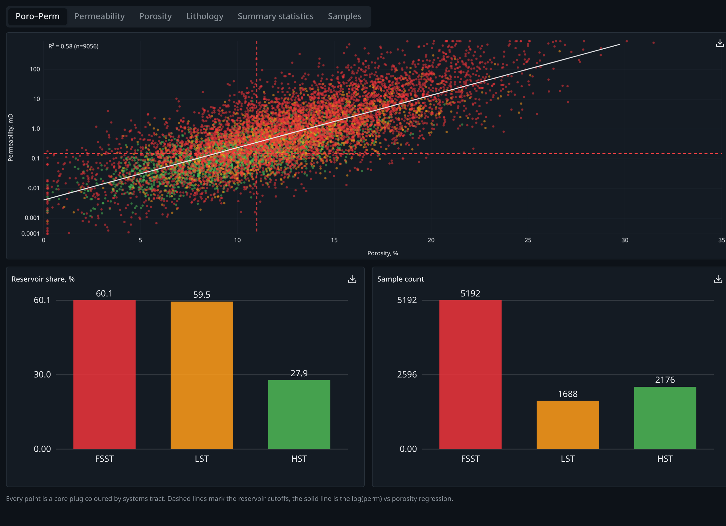
Two things matter in a plot like this. First, the tract populations must separate — if they do not, either the markers are wrong or the interval is genuinely uniform. Second, the position of each population relative to the cutoffs is the practical answer: the regressive tracts sit above and to the right of the cutoff cross, the transgressive material below and to the left.

In GeoSequence: Open the core module, load the demo set or import your own CSV/XLSX, then assign tracts from the log interpretation or from seismic zones and filter by tract, well or unit. open the module →

The summary statistics table condenses the crossplot into numbers an evaluation can use: arithmetic and geometric means, modes, P90 permeability, and — most useful for volumetrics — the share of plugs that pass the cutoffs, plus the average properties of only those net-reservoir plugs.

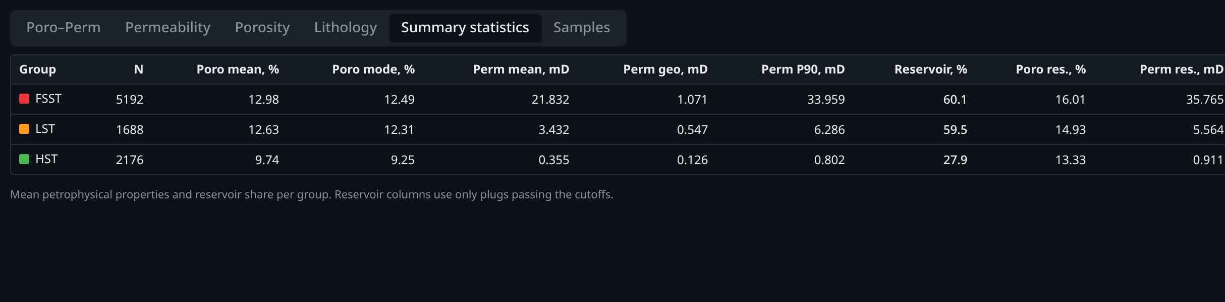
Read together, tract, facies and petrophysics form a single ranked table. It is worth building explicitly for every field, because the ranking is what gets carried into the seismic domain in section 05.

Between the tract and the plug sits the facies. Curve-shape analysis (the Muromtsev electrometric approach, and its Western equivalents) reads the gamma-ray envelope of a single body: funnel-shaped coarsening-upward for shoreface and delta front, bell-shaped fining-upward for channel fill and transgressive lags, cylindrical for aggrading braided or amalgamated turbidites, irregular for reworked forced-regression deposits.

In exploration terms the shapes matter because they carry geometry: a funnel body is a broad, laterally continuous belt parallel to the palaeoshoreline, while a bell body is a narrow, sinuous channel. The same net-to-gross means very different drainable volume in the two cases.

In GeoSequence: Run wavelet cycle detection, then the facies module to classify curve shapes and plays automatically, and cross-check them against tract boundaries on the tablet. open the module →

Wells calibrate; seismic distributes. Once the horizons that bound a tract are tracked, the interval between them can be characterised by amplitude, frequency and continuity attributes, and the tract becomes a zone with internal facies belts. A stratal (sedimentation) slice inside that zone shows the depositional system in map view instead of a time slice cutting across it.

• Amplitude and RMS in the zone track sand thickness and net-to-gross within the fairway.
• Frequency and bandwidth separate thick amalgamated bodies from thin interbedded ones.
• Continuity and semblance outline channels, lobes and erosional edges.
• Wheeler and Railway transforms reveal where the tract is missing entirely — hiatus and truncation are exploration risk, not just a display artefact.

In GeoSequence: Track horizons with live autocorrelation, type them as erosion / SB / intrusion, auto-detect tract zones between picks, then inspect them in 3D, Wheeler and stratal-slice views. open the module →

A sweet spot is the intersection of three independent maps, not one favourable attribute. In sequence-stratigraphic terms it is the part of a reservoir-prone tract where (1) the seismic facies belt is the depositional fairway, (2) core-calibrated properties clear the cutoffs, and (3) seal and charge from the neighbouring transgressive interval are intact.

Practically the workflow is a stack of thresholded grids: net reservoir share from core statistics per tract, an attribute-based facies class from the seismic zone, tract thickness from the horizon pair, and a seal-presence flag from the overlying TST. Ranking the intersection produces drillable targets with an explicit geological argument behind each one, which is what a partner or a licence round actually asks for.

1. Load logs, lithology and core; run QC and unit conversion.
2. Build the age–depth stratigraphic framework.
3. Detect cycles (wavelet), pick SB / TS / MFS, compute tracts by Vail, Catuneanu or Muromtsev.
4. Classify curve-shape facies and plays.
5. Assign tracts to core plugs; check that the crossplot populations separate and record net reservoir share per tract.
6. Track seismic horizons, type them, auto-detect tract zones and extract facies attributes.
7. Intersect fairway, calibrated quality, thickness and seal to rank sweet spots; export maps and tables.

Pitfalls worth naming

• Circular calibration. Do not assign tracts to core from seismic zones and then use the core to validate those zones. Keep at least one independent control.
• Plug bias. Cored intervals are usually chosen because they look good; net reservoir share from core is an optimistic estimate unless coverage is checked per tract.
• Diagenetic overprint. Depositional facies predicts initial quality only. Cementation and compaction can invert the tract ranking at depth — always plot properties against depth as well as tract.
• Tuning and resolution. A tract thinner than a quarter-wavelength cannot be mapped as a zone; use the Wheeler view to distinguish real hiatus from a package below resolution.
• TWT vs depth. Thickness-driven conclusions require a depth volume or a reliable velocity model; forced regression wedges are especially sensitive to this.

For the methods themselves — base level and A/S, the Vail and Catuneanu models, wavelet cycles and Wheeler transforms — see part 1 of the guide.